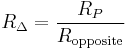
Y-Δ transform
The Y-Δ transform, also written wye-delta and known by many other names, is a mathematical technique to simplify the analysis of an electrical network. The name derives from the shapes of the circuit diagrams, which look respectively like the letter Y and the Greek capital letter Δ. This circuit transformation theory was published by Arthur Edwin Kennelly in 1899.[1]
Contents |
Names
[[Image:Theoreme de kennelly.png|right|thumb|400px|Illustration of the transform in its T-Π representation, ]
The Y-Δ transform is known by a variety of other names, mostly based upon the two shapes involved, listed in either order. The Y, spelt out as wye, can also be called T or star; the Δ, spelt out as delta, can also be called triangle, Π (spelt out as pi), or mesh. Thus, common names for the transformation include wye-delta or delta-wye, star-delta, star-mesh, or T-Π.
Basic Y-Δ transformation
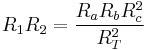
The transformation is used to establish equivalence for networks with three terminals. Where three elements terminate at a common node and none are sources, the node is eliminated by transforming the impedances. For equivalence, the impedance between any pair of terminals must be the same for both networks. The equations given here are valid for complex as well as real impedances.
Equations for the transformation from Δ-load to Y-load 3-phase circuit
The general idea is to compute the impedance  at a terminal node of the Y circuit with impedances
  ,
,  to adjacent nodes in the Δ circuit by
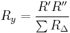
where  are all impedances in the Δ circuit. This yields the specific formulae
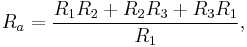
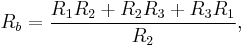
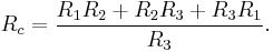
Equations for the transformation from Y-load to Δ-load 3-phase circuit
The general idea is to compute an impedance in the Δ circuit by
where  is the sum of the products of all pairs of impedances in the Y circuit and
  is the impedance of the node in the Y circuit which is opposite the edge with . The formula for the individual edges are thus
Usefulness
Resistive networks between two terminals can theoretically be simplified to a single equivalent resistor (more generally, the same is true of impedance). Series and parallel transforms are basic tools for doing so, but for complex networks such as the bridge illustrated here, they do not suffice.
The Y-Δ transform can be used to eliminate one node at a time and produce a network that can be further simplified, as shown.
The reverse transformation, Δ-Y, which adds a node, is often handy to pave the way for further simplification as well.
Graph theory
In graph theory, the Y-Δ transform means replacing a Y subgraph of a graph with the equivalent Δ subgraph. The transform preserves the number of edges in a graph, but not the number of vertices or the number of cycles. Two graphs are said to be Y-Δ equivalent if one can be obtained from the other by a series of Y-Δ transforms in either direction. For example, the Petersen graph family is a Y-Δ equivalence class.
Demonstration
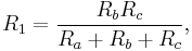
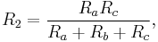
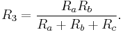
Δ-load to Y-load transformation equations
To relate 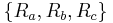 from Δ to
 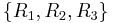 from Y, the impedance between two corresponding nodes is compared. The impedance in either configuration is determined as if one of the nodes is disconnected from the circuit.
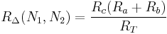
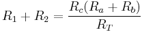
The impedance between N1 and N2 with N3 disconnected in Δ:
![\begin{align}
R_\Delta(N_1, N_2) &= R_c \parallel (R_a%2BR_b) \\[8pt]
&= \frac{1}{\frac{1}{R_c}%2B\frac{1}{R_a%2BR_b}} \\[8pt]
&= \frac{R_c(R_a%2BR_b)}{R_a%2BR_b%2BR_c}.
\end{align}](/2012-wikipedia_en_all_nopic_01_2012/I/5592b55a9e9ff1c8454c332c7ca50e9d.png)
To simplify, let  be the sum of .
Thus,
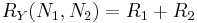
The corresponding impedance between N1 and N2 in Y is simple:
hence:
 (1)
(1)
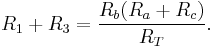
Repeating for  :
:
 (2)
(2)
and for  :
:
 (3)
(3)
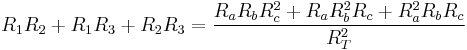
From here, the values of can be determined by linear combination (addition and/or subtraction).
For example, adding (1) and (3), then subtracting (2) yields

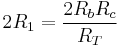
thus,
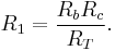
where 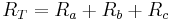
For completeness:
 (4)
(4)
 (5)
(5)
 (6)
(6)
Y-load to Δ-load transformation equations
Let
- .
We can write the Δ to Y equations as
- (1)
- (2)
 (3)
(3)
Multiplying the pairs of equations yields
 (4)
(4)
 (5)
(5)
 (6)
(6)
and the sum of these equations is
 (7)
(7)
Factor  from the right side, leaving in the numerator, canceling with an in the denominator.
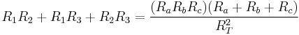
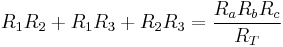 (8)
(8)
-Note the similarity between (8) and {(1),(2),(3)}
Divide (8) by (1)
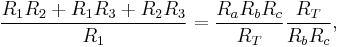
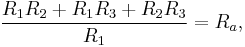
which is the equation for  . Dividing (8) by (2) or (3) (expressions for
  or
or  ) gives the remaining equations.
See also
- Analysis of resistive circuits
- Electrical network, single-phase electric power, alternating-current electric power, three-phase power, polyphase systems for examples of Y and Δ connections
- AC motor for a discussion of the Y-Δ starting technique
- Nikola Tesla
- John Hopkinson
- Mikhail Dolivo-Dobrovolsky
- Charles Proteus Steinmetz
Notes
- ^ A.E. Kennelly, Equivalence of triangles and stars in conducting networks, Electrical World and Engineer, vol. 34, pp. 413–414, 1899.
References
- William Stevenson, Elements of Power System Analysis 3rd ed., McGraw Hill, New York, 1975, ISBN 0070612854
External links
- Star-Triangle Conversion: Knowledge on resistive networks and resistors
- Calculator of Star-Triangle transform